
Measurement Uncertainty in Industrial Sensor Systems
Measurement uncertainty is a non-negative parameter that characterises the dispersion of quantity values attributed to a measurand, based on the information used. In industrial sensor systems it brings together uncertainty from the sensor, calibration, signal conditioning, data acquisition, environment, installation and measurement method.
Uncertainty is not the same as error, tolerance or resolution. The evaluation starts with a defined measurand and measurement model, then standardises and propagates the relevant contributions before any expanded uncertainty is reported.

Do not add datasheet percentages directly. First express every relevant contribution as a standard uncertainty in the output quantity, apply sensitivity coefficients and correlations where required, then combine the components and state the coverage used for the reported result.
Uncertainty describes the quality of a measurement result, not a mistake in the reading
A measured value is an estimate of a measurand. Even after known significant systematic effects have been corrected, incomplete knowledge remains: the reference standard has uncertainty, repeated readings vary, sensor characteristics change with temperature, the analogue chain adds noise and drift, and the measurement model may depend on quantities that are themselves not known exactly.
| Term | Meaning | Do not confuse it with |
|---|---|---|
| Measurement error | Difference between a measured quantity value and a reference quantity value. The exact error is normally not fully known in a real measurement. | Uncertainty. Error can have sign; uncertainty is a non-negative parameter. |
| Standard uncertainty, u | Measurement uncertainty expressed as a standard deviation. | A tolerance or maximum permissible error. |
| Combined standard uncertainty, uc | Standard uncertainty of the output quantity after relevant input uncertainties are propagated through the measurement model. | A simple arithmetic sum of specifications. |
| Expanded uncertainty, U | Combined standard uncertainty multiplied by a coverage factor k to provide an interval with a stated coverage interpretation. | An automatic 95% interval for every case. |
| Uncertainty budget | Structured list of uncertainty sources, distributions, standard uncertainties, sensitivity coefficients and contributions. | A list of every datasheet tolerance without a measurement model. |
Build the uncertainty budget around the actual sensor-to-result measurement chain
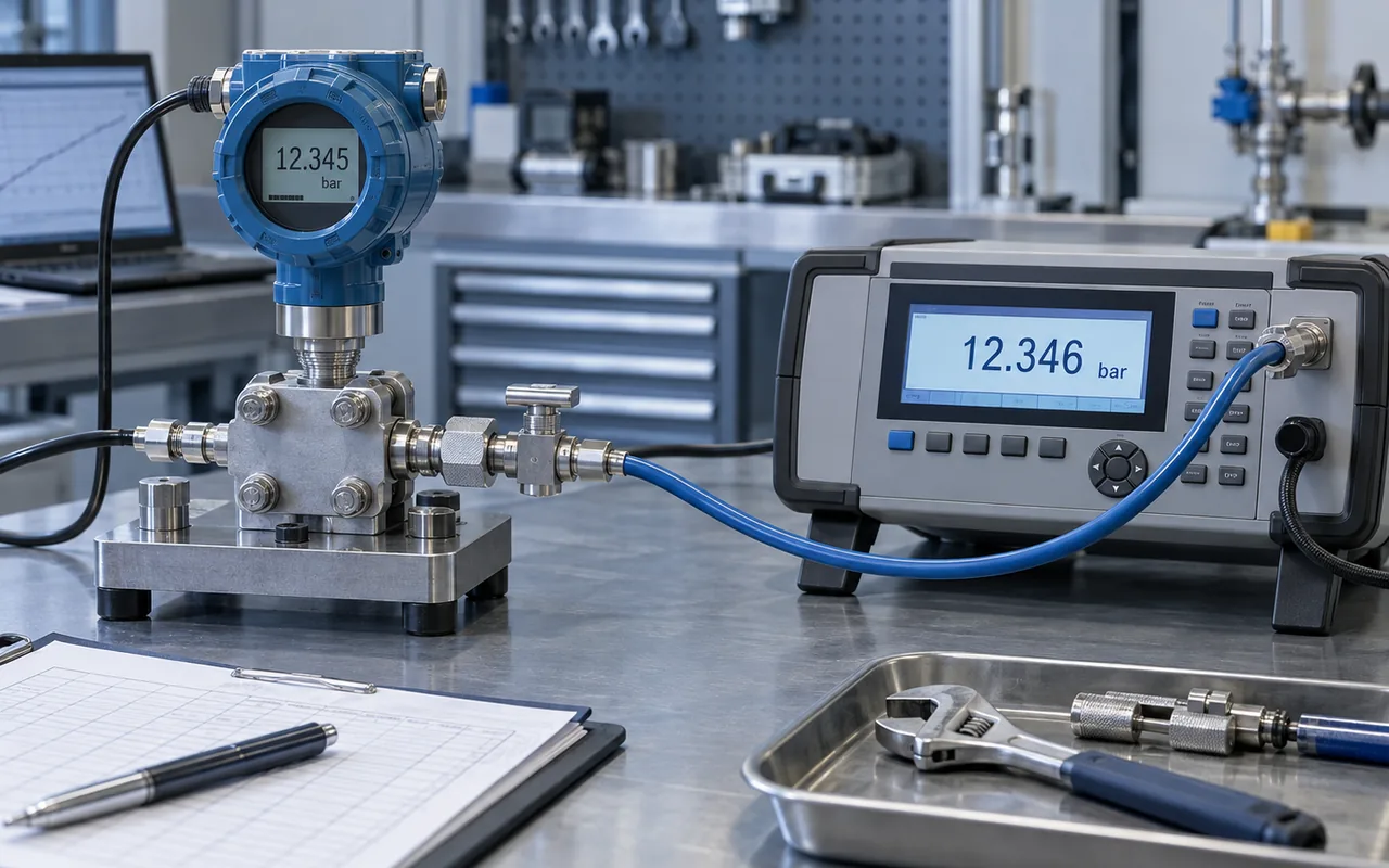
There is no universal list of uncertainty terms that applies unchanged to every sensor. The budget should follow the measurement model and the conditions of use. A pressure measurement, for example, may include a calibrated reference, transmitter repeatability, ambient-temperature influence, mounting effects, signal-conditioning gain, ADC reference error and the repeatability of the complete reading.
Calibration uncertainty, repeatability, hysteresis, zero stability, temperature influence, cross-sensitivity and installation effects.
Gain and offset uncertainty, reference stability, bridge excitation, CJC, isolation amplifier behaviour, filtering and input-referred noise.
Input range, reference uncertainty, conversion noise, linearity, channel crosstalk, sampling effects and resolution where it is actually significant.
Temperature, humidity, vibration, electromagnetic interference, cable thermal effects, pressure head, self-heating and power-supply variation.
Calibration-certificate uncertainty, drift since calibration, resolution of the reference, transfer method and stability during the comparison.
Alignment, mounting, corrections, operator influence, mathematical model, fluid density, lead resistance, sampling window and data reduction.
Do not automatically include the full specified accuracy of every component if a calibration of the complete chain already characterises the same effect. Conversely, do not omit a relevant environmental or installation term merely because it is absent from the sensor's headline accuracy specification. The goal is to avoid both double counting and missing contributions.
Type A and Type B describe how a standard uncertainty is evaluated
A Type A evaluation obtains a standard uncertainty by statistical analysis of a series of observations. A Type B evaluation uses other information, such as calibration certificates, manufacturer data, previous measurements, reference data, resolution limits or engineering knowledge. Type A and Type B do not mean random and systematic error, and there are no “Type A errors” or “Type B errors”.
Type A: repeated observations
If n repeated readings are made under defined conditions, their statistical spread can be used to estimate an uncertainty component. When the measurand is represented by the mean, the relevant standard uncertainty of that mean commonly depends on the sample standard deviation and the number of independent observations.
Type B: other available information
Type B evaluation uses information other than a Type A statistical analysis of the current series of observations and expresses the resulting component as a standard uncertainty. Examples include a calibration certificate with stated expanded uncertainty, a manufacturer limit, a known resolution step, a temperature coefficient applied over an estimated temperature range, or prior knowledge of a reference standard's drift.
The probability distribution should represent the information available; it should not be selected only because it gives a smaller number.
Convert limits and certificate statements to standard uncertainties before combining them
Specifications arrive in different forms: ± limits, standard deviations, confidence intervals, resolution steps and expanded uncertainties. They cannot be combined consistently until they are expressed as standard uncertainties and referred to the same output quantity.
| Available information | Typical model | Standard uncertainty |
|---|---|---|
| Standard deviation stated directly | Normal or empirical distribution | Use the stated standard deviation when it represents the quantity required by the model. |
| Expanded uncertainty U with coverage factor k | Certificate statement | u = U / k |
| Symmetric limit ±a with no reason to prefer values inside the interval | Rectangular distribution | u = a / √3 |
| Symmetric limit ±a with values near the centre more likely and linearly decreasing probability | Triangular distribution | u = a / √6 |
| Digital step or quantisation interval q, rounding assumed within ±q/2 | Rectangular quantisation | u = q / √12 |
For sensor datasheets, identify the percentage basis before converting a specification. On a 0–10 bar range, ±0.1% of full scale is ±0.010 bar, whereas ±0.1% of a 6.20 bar reading is ±0.0062 bar. Percent of span and percent of reading are not interchangeable, and the resulting limit still needs an appropriate probability model before it is treated as a standard uncertainty.
Propagate uncertainty through the measurement model, including sensitivity and correlation
Suppose the measurement result y is calculated from input quantities x1, x2, … through a measurement model y = f(x1, x2, …). Each input uncertainty affects the result according to a sensitivity coefficient ci, which describes how much the output changes when that input changes.
For a simple additive model, a sensitivity coefficient may be 1. For scaling or nonlinear models it may be a conversion factor or a derivative of the output with respect to the input quantity. This is why simply adding percentages from different parts of a system is often wrong: the contributions may be in different units and may not affect the result equally.
Uncorrelated contributions
Independent standard uncertainty contributions are commonly combined by RSS after each has been converted to the output quantity. A single dominant contribution will largely determine the result; many very small terms may have negligible effect.
Correlated contributions
Correlation matters when two inputs share the same reference, environment, calibration source, excitation or processing path. Positive correlation can increase combined uncertainty; negative correlation can reduce it. Treating correlated terms as independent can materially misstate the result.
Use a coverage factor only after the combined standard uncertainty is established
Expanded uncertainty is obtained from the combined standard uncertainty using a coverage factor:
A coverage factor of k = 2 is often associated with a coverage probability of approximately 95% when the conditions for that interpretation are reasonable, such as an approximately normal output distribution with sufficient effective degrees of freedom. It is not a universal identity. Small samples, strongly non-normal distributions, dominant Type B rectangular terms or nonlinear measurement models can require a different treatment. Where important components have limited degrees of freedom, an effective degrees-of-freedom estimate such as the Welch–Satterthwaite approximation can be used to select an appropriate Student t coverage factor.
A simple pressure-measurement budget shows why the largest contributor matters most
Consider a 0–10 bar measurement chain producing a result near 6.20 bar. Assume the relevant effects have already been corrected where appropriate and the following remaining contributions are reasonable for the actual operating conditions. The numbers are illustrative, but the method is the same for real budgets.
| Source | Basis | Standard uncertainty at result |
|---|---|---|
| Reference calibration | Certificate standard uncertainty | 0.012 bar |
| Complete-chain repeatability | Type A evaluation | 0.006 bar |
| Displayed resolution | 0.002 bar step, rectangular rounding | 0.00058 bar |
| Residual temperature influence | ±0.015 bar rectangular limit | 0.00866 bar |
| Conditioning / acquisition | Combined input-referred contribution | 0.004 bar |
If these terms are reasonably treated as uncorrelated, their RSS combination gives a combined standard uncertainty of about 0.0165 bar. Using k = 2 gives an expanded uncertainty of about 0.033 bar.
The reference and temperature contributions dominate this example. Improving a 0.002 bar display step would barely change the total uncertainty, while improving the reference or temperature compensation could have a visible effect. An uncertainty budget therefore helps prioritise engineering effort instead of simply buying more ADC bits.
Report enough information for another engineer to interpret the uncertainty statement
A useful measurement uncertainty statement identifies the measured result and unit, states whether the quoted uncertainty is standard or expanded, gives the coverage factor when expanded uncertainty is used, and documents the measurement model and important assumptions well enough for the result to be interpreted. The number of digits in the result should be consistent with the uncertainty; false precision should be avoided.
- Define the measurand. Specify exactly what quantity is being measured, under what conditions and at what point in the process.
- Apply known corrections. A recognised significant systematic effect should normally be corrected rather than hidden inside a large uncertainty allowance.
- List relevant inputs. Include sensor, reference, conditioning, acquisition, environmental, installation and method terms that materially influence the result.
- Standardise each contribution. Convert limits and certificate statements into standard uncertainties and propagate them to the output quantity.
- Check correlation. Shared references, excitation, environmental variables and common calibration data can make terms dependent.
- Combine and expand. Calculate uc, then apply a justified k only if expanded uncertainty is required.
- Review dominance. Focus improvement on the largest meaningful contributors instead of uniformly tightening every component specification.