0–10 V Sensor Cable Length: Voltage Drop & Wiring Limits
A 0–10 V sensor has no single cable-length limit. Cable resistance, the shared common, output loading and electrical noise all matter. Start with the sensor manufacturer’s cable limit and the receiving input’s specifications.
A three-wire sensor can have enough supply voltage and still give a wrong reading at the programmable logic controller (PLC).
Use the one-way length for each cable core. The signal wire carries the input current, not the sensor’s full operating current.
How far can a 0–10 V sensor cable run?
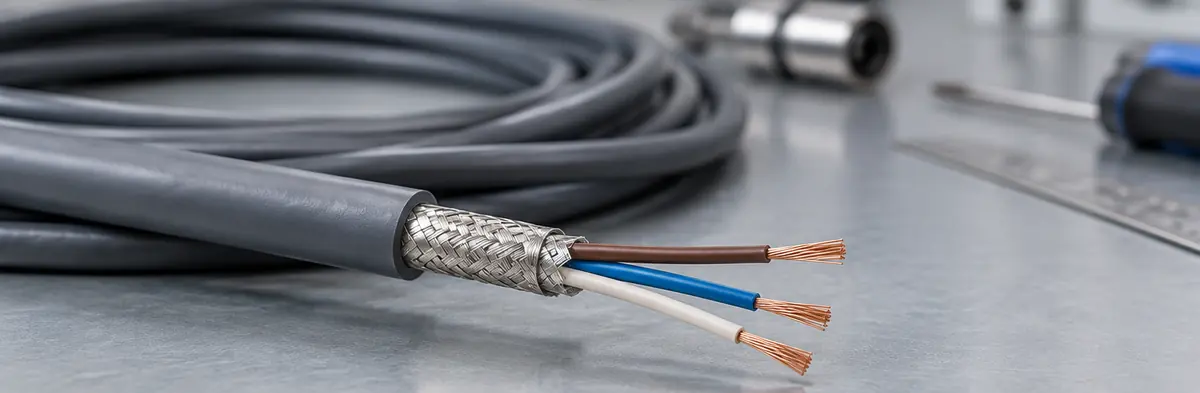
The sensor’s installation manual takes priority. A cable run within its stated limit still needs to meet the accuracy requirement of the measurement. Check the resistance of the conductors, the PLC input resistance and the cable route before choosing a length.
Balluff gives 50 ft (about 15 m) as a general guide for analogue voltage signals, assuming a correctly terminated shielded cable routed away from high-energy AC sources. It also notes that longer runs are possible. This is a manufacturer’s guideline, not a limit defined by the 0–10 V interface. [1]
| Find this specification | Where to look | What it decides |
|---|---|---|
| Minimum operating supply and current consumption | Sensor datasheet, including the selected output mode | Whether the voltage remaining at the sensor supports its specified output range. |
| Minimum load resistance, output-current limit and capacitive-load limit | Sensor output specification | Whether the output can drive the receiving input and cable. A minimum load resistance is not the sensor’s output resistance. |
| Input resistance and input/reference arrangement | PLC or controller analogue-input manual | Loading error, common-mode limits and whether a separate reference lead can be used. |
| Resistance per conductor, capacitance and permitted installation conditions | Cable datasheet | Conductor losses and compatibility with the output. Use resistance appropriate to operating temperature. |
| Allowed wiring error | Measurement requirements or uncertainty budget | How much error remains available after the sensor and input errors are allowed for. |
Use the one-way cable length when calculating a single conductor’s resistance. Add the outward and return resistances only for a path that actually includes both conductors.
Supply loss, loading and common-wire error
The following model is for a powered three-wire sensor: supply, voltage output and a shared power/signal common. The cabinet supply negative and the single-ended analogue-input common are connected together. Wire colours and connector pins vary; use the device wiring diagram.
A long cable can make a 0–10 V reading too high, not just too low. In the shared-common connection above, the PLC measures the sensor output plus the rise in sensor-common potential, with output loading also present. Campbell Scientific documents this mechanism in powered voltage-output sensors. [2]
NI’s input-impedance explanation describes the separate voltage-divider effect. Do not use the sensor’s operating current to calculate the signal-core drop: the input draws its own, usually much smaller, current. [3]
0–10 V cable-error calculator
Enter the actual cable and device values. This model assumes three equal-resistance conductors, a resistive single-ended input and no parallel common or earth paths. It estimates DC resistance effects; it does not calculate a guaranteed maximum cable length.
I₀ is the current returning through the sensor’s common wire, not its signal wire. Use the value for the operating mode being checked. When only total supply current is listed, using that value gives a conservative estimate for this circuit because some supply current returns through the PLC input.
The defaults describe the example below, not a named product. The result excludes sensor and PLC accuracy, leakage, output clipping, changes in operating conditions, cable capacitance and interference.
Equations and circuit assumptions
The equations below are derived from Ohm’s law and the voltage divider for the stated circuit. They do not describe every three-wire output. The sensor supply provides both I₀ and the signal current; only I₀ returns in the common core.
- L, r
- One-way length in metres and single-core resistance in Ω/km.
- R
- Resistance of each of the three equal cable cores.
- E, Rₒ, Rᵢ
- Unloaded local source voltage, equivalent output resistance and input resistance.
- I₀, G, k
- Common-return current in amperes, common-potential rise and voltage-divider factor.
- Vᵢ, Iᵢ, Vₛ
- Voltage at the input, input current and cabinet supply voltage.
Iᵢ = Vᵢ / Rᵢ
The bound adds the magnitudes of the loading and common-wire errors. It is a conservative design allowance, not the exact maximum error: the two effects partly cancel in this circuit. I₀ and Rₒ are assumed constant across 0–10 V; repeat with their worst-case values when they vary. The supply check includes the 10 V endpoint and assumes an output without internal voltage boosting.
For unequal conductors, use the actual common resistance in G, the actual signal resistance in k and the positive-core resistance in the supply equation. Do not add another return-core resistance to this divider: the common-core effect has already been included through G for this topology.
50 m example: enough supply voltage, too much signal error
Consider a 50 m (164 ft) run with a resistance of 60 Ω/km per core, 20 mA in the common core, a 5.000 V unloaded signal, 50 Ω equivalent output resistance and a 100 kΩ input. The cabinet supply is 24 V; the assumed sensor minimum is 10 V.
Common rise = 0.020 A × 3 Ω = 0.060 V
PLC input = (5.000 + 0.060) × 100000 / 100053 ≈ 5.0573 VThree equal-resistance cores, a shared power/signal common and a resistive single-ended input.
The supply remaining at the sensor is about 23.880 V, above the assumed minimum. Yet the input reads about 57.32 mV high: 0.5732% of the 10 V span. On a linear 0–100 bar transmitter, that would represent about 0.573 bar of additional indicated pressure.
Adding the maximum loading loss to the common-wire contribution gives a conservative bound of 65.265 mV, or 0.6527% of span. This is above the 0.5% wiring-error budget, before adding sensor and PLC errors.
| One-way run | Resistance per core | Common rise | Conservative error bound |
|---|---|---|---|
| 10 m / 33 ft | 0.60 Ω | 12.0 mV | 0.1705% span |
| 25 m / 82 ft | 1.50 Ω | 30.0 mV | 0.3513% span |
| 50 m / 164 ft | 3.00 Ω | 60.0 mV | 0.6527% span |
| 100 m / 328 ft | 6.00 Ω | 120.0 mV | 1.2553% span |
All other example values stay fixed. This is a comparison of resistance effects, not an approved cable-length table. At zero cable length, the assumed 50 Ω output resistance still causes loading; the calculation includes that source/input contribution.
Cable length for a common-wire error limit
When input loading is small, the common-wire contribution is approximately I₀ × Rcommon. A first estimate of the length that would use an allocated common-wire voltage error is:
Allowing 20 mV, or 0.2% of a 10 V span, with 20 mA return current and 0.06 Ω/m gives about 16.7 m (55 ft). This is the common-wire budget only. Other errors and the manufacturer’s requirements can demand a shorter run or a different connection.
A thicker common conductor reduces this particular error. For example, halving its resistance halves I₀ × Rcommon at unchanged current. Increasing only the positive-supply conductor does not remove the common-reference shift. Improving the cable shield does not reduce this DC resistance either.
Cable capacitance and electrical noise
Cable capacitance loads the output during voltage changes. A high DC input resistance does not remove that load. Check the sensor’s capacitive-load limit: an unsuitable load can slow the response or make an active output unstable. [5]
For an illustrative cable capacitance of 100 pF/m, a 50 m run contributes 5 nF for the specified conductor configuration, before connector and input capacitance. Use capacitance specified for the same conductor configuration; core-to-shield and core-to-core values are not interchangeable.
Route signal wiring away from motor leads and variable-frequency-drive output cables as required by the equipment instructions. Follow the specified twisting, shielding and bonding arrangement. A shield connection is an EMC design choice, not a universal “one end only” rule, and the shield should not substitute for the required signal common. [4]
Observe the signal while the equipment is running, including when nearby loads switch. A multimeter can miss brief disturbances. For waveform checks, use an oscilloscope or recorder with the correct probe isolation and input-voltage ratings.
Check supply and signal at both ends
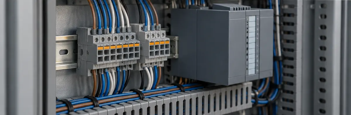
Keep the measured quantity steady while comparing readings. Record both test points for every voltage measurement: changing the reference terminal changes what the voltage means.
These checks are for trained personnel working under the site’s safe-working procedure. Isolate before changing connections. Use appropriately rated instruments; never place a multimeter set to current across a voltage output or supply.
- Measure supply at the sensor while it is operating. Measure between the sensor’s own +V and 0 V terminals, not between cabinet terminals. Repeat under the highest expected current demand.
- Measure the local signal. Record VOUT relative to the sensor’s specified signal common with the receiving input connected. This is the loaded terminal voltage, not necessarily the calculator’s unloaded source E.
- Measure at the receiving input. Record AI+ relative to the channel’s specified common or negative input. Verify the channel’s voltage mode and compare its displayed voltage or raw value with the meter.
- Check the common-potential difference. With an approved measurement method, compare sensor common with cabinet common. A voltage that changes with sensor operating current points towards a shared-return contribution.
- Test more than one signal level. Check the low, middle and high parts of the range. A nearly constant offset, a proportional loading error and a supply-limited output need different corrections.
- Repeat with relevant machinery running. Intermittent disturbances that follow a drive, contactor or other load suggest a routing, reference or EMC issue rather than a fixed cable-resistance error.
| Observation | Next check |
|---|---|
| Sensor supply is below its operating minimum | Supply setting, conductor resistance, connections and current demand. Resolve this before trusting the signal calculation. |
| PLC voltage is higher than the local loaded signal | Common-potential rise and other reference paths. Measure rather than assume the sign of the error. |
| Connecting the input reduces the local sensor voltage | Input mode, input resistance and the sensor’s load rating. An input configured for current may load a voltage output incorrectly. |
| Meter at the input is correct, but engineering units are wrong | Channel range, raw-count conversion and engineering limits. See 0–10 V scaling. |
| Reading changes mainly when adjacent equipment switches | Routing, bonding, input reference, isolation and transient interference. |
Reduce the error or change the connection
| Change | What it can address | What still needs checking |
|---|---|---|
| Shorter run or lower-resistance conductors | Supply drop and common-wire voltage rise. | Output loading, capacitance and EMC. There is no fixed distance gain independent of the circuit. |
| Separate signal-reference lead to a compatible differential input | Keeping operating-current drop out of the sensed reference path. | Permitted sensor wiring, input bias paths and common-mode range. Merely selecting “differential” at the cabinet does not bypass the same shared conductor. |
| Local signal conditioning or isolation | Input loading or ground-potential differences. | Conditioner location, reference wiring, accuracy, supply and bandwidth. A conditioner receiving an already incorrect voltage cannot recover the original signal. |
| Compatible 4–20 mA transmission or remote I/O | Moving away from a long single-ended voltage connection. | Loop-voltage budget or network limits, power, diagnostics and the receiver. Changing a PLC menu does not convert a 0–10 V sensor into a current transmitter. |
A separate signal-reference lead can keep power-return voltage drop out of the measurement. The differential input must still remain within its common-mode range. [2] [4]
Compare 4–20 mA and 0–10 V before changing the interface. The signal-conditioning guide covers buffering, filtering and isolation.
0–10 V cable-length questions
Can I run a 0–10 V sensor over 100 m?
Only if the sensor, cable and receiving input support it. Check the manufacturer’s cable and load limits, calculate supply and common-wire losses, and test the installed signal. The 100 m row above compares resistance effects; it does not approve that length for any specific sensor.
Will a higher supply voltage improve the 0–10 V reading?
It can restore operation when the sensor was underpowered, provided the new supply is within its rating. At unchanged current, it does not remove I₀ × Rcommon or the output/input loading ratio. Increasing supply voltage is not a general signal-error correction.
Can I compensate for cable error in PLC scaling?
A verified, repeatable offset or gain error can sometimes be included in calibration. First correct wiring and loading faults. A correction made at one operating current or temperature may be wrong at another, and scaling does not eliminate electrical noise, clipping or inadequate sensor supply.
What if the sensor datasheet does not give output resistance?
Use its specified load range and accuracy conditions; ask the manufacturer for clarification when necessary. Do not enter the minimum load resistance as output resistance. The calculator’s zero-resistance setting isolates other effects under an ideal-source assumption, but cannot prove total accuracy.
Is this also a calculator for 0–10 V lighting dimming?
No. This model is for a sensor driving a voltage input, not a dimmer connected to a lighting driver. Use the lighting equipment’s cable and installation limits.
Technical sources
- Balluff. Maximum cable lengths for analog sensors. Scott Rosenberger, 18 June 2024. General distance recommendations and installation conditions.
- Campbell Scientific. How do long cable lengths affect measurements? FAQ, Voltage Measurements. Shared power/signal return and separate-reference measurements.
- NI. Specifications Explained: C Series Modules. Input Impedance section. Resistive loading of a voltage source.
- NI. Field Wiring and Noise Considerations for Analog Signals. Updated 15 August 2024. Input referencing, common-mode limits and noise coupling.
- Analog Devices. Stability 101: Driving a Capacitive Load (Operational Amplifiers). Matt Duff, 12 September 2012. Output-stage stability with capacitive loads.
Product-specific supply, load, EMC and installation limits take precedence over these illustrative calculations.